Machine learning

at the intersection of statistics and artificial intelligence

algorithms for inferring unknowns from unknowns

ML Model

A Model is a description of possible data one could observe

Generative Models

To get the conditional probability P(Y|X), generative models estimate the prior P(Y) and likelihood P(X|Y) from training data and use Bayes rule to calculate the posterior P(Y |X):

we have a notion of the underlying distribution of the data and we want to find the hidden parameters of that distribution. Some approaches are:

• Naive Bayes classifiers,
• Gaussian mixture models,
• variational autoencoders,
• generative adversarial networks and others.

Discriminative Models

discriminative models directly assume functional form for P(Y|X) and estimate parameters of P(Y|X) directly from training data. They are more suitable when we only want to find the boundary that separates the data into different classes.

• support vector machines
• logistic regression (LR),
• perceptron

Python modules

There are multiple modules for machine learning in python, which you will regularly use alongside moddules like numpy, scipy, and pandas

• sckit-learn: https://scikit-learn.or
• theano: https://github.com/Theano/Theano --> (https://github.com/pymc-devs/aesara)
• pytorch: https://pytorch.org/
• tensorflow: http://tensorflow.org/
• keras: https://keras.io/

import matplotlib.pyplot as plt
import numpy as np
color = ['#377eb8', '#ff7f00', '#4daf4a',
         '#f781bf', '#a65628', '#984ea3',
        '#999999', '#e41a1c', '#dede00']

Supervised learning

given a some data (Xi,Yi)...(Xn, Yn), choose a function f(x) that takes a (new) data point X and gives you a Y. This is an illposed problem. Very difficult to do unless by making certain assumptions

• Classification: Yi belong to one finite set
• Regression: Y belong to R, or R**d

Regression

Suppose that Xi are real valued, and Yi are real valued

N = 30
xc = np.random.random((2,N))
# fake tendency line
tendency = np.linspace(-1,1,N) 
xc *= tendency
plt.scatter(xc[0],xc[1], color='b')

<matplotlib.collections.PathCollection at 0x7f7d8be01390>

Given an X, figure out what Y is associated to that value. Function that returns values for any given X.

from sklearn.linear_model import LinearRegression 
linear_regressor = LinearRegression()  # create object for the class
plt.scatter(xc[0],xc[1], color='b')
estimate = linear_regressor.fit(xc[0].reshape(-1,1), xc[1].reshape(-1,1))  # perform linear regression
pred = linear_regressor.predict(xc[0].reshape(-1,1))  # make predictions
plt.plot(xc[0], pred, color='r')

[<matplotlib.lines.Line2D at 0x7f7d74b3ef50>]

Classification

Suppose we have 20 data points in two dimensions (x1, x2) with two classes/labels (y1, y2)

a = (np.random.random(20) * 0.1 + 0.4, np.random.random(20) * 0.1 + 0.4)
b = (np.random.random(20) * 0.1 + 0.3, np.random.random(20) * 0.1 + 0.3)
plt.scatter(a[0],a[1],c=color[0],label='A')
plt.scatter(b[0],b[1],c=color[1],label='B')
plt.legend()

<matplotlib.legend.Legend at 0x7f7d74a9de50>

Unsupervised learning

Given some data (x1,...,xn), find patterns in data (whatever that means)

some types of patterns:

• Clustering
• Density estimation
• Dimensionality reduction

Clustering

Given some points in two dimensional real space (R2), find groups of clusters on the data

from sklearn.datasets.samples_generator import make_blobs

X, _ = make_blobs(n_samples=300, centers=4,
                       cluster_std=0.60, random_state=0)

plt.scatter(X[:, 0], X[:, 1], s=50);

/usr/local/lib/python3.7/dist-packages/sklearn/utils/deprecation.py:144: FutureWarning: The sklearn.datasets.samples_generator module is  deprecated in version 0.22 and will be removed in version 0.24. The corresponding classes / functions should instead be imported from sklearn.datasets. Anything that cannot be imported from sklearn.datasets is now part of the private API.
  warnings.warn(message, FutureWarning)

from sklearn.cluster import KMeans
kmeans = KMeans(n_clusters=4)
kmeans.fit(X)
y_kmeans = kmeans.predict(X)

plt.scatter(X[:, 0], X[:, 1], c=y_kmeans, s=50, cmap='viridis')

centers = kmeans.cluster_centers_
plt.scatter(centers[:, 0], centers[:, 1], c='pink', s=200, alpha=0.9);

Linear Classification

Perceptron

data = np.random.random((100,2))

print(data[:2])

[[0.19631142 0.54006566]
 [0.65221156 0.49457156]]

labels = np.where(data[:,0] > data[:,1], 1, -1)

print(labels, labels.shape)

[-1  1 -1  1 -1 -1 -1 -1 -1 -1 -1 -1  1 -1 -1 -1 -1  1 -1 -1  1  1 -1  1
 -1  1 -1 -1  1 -1 -1 -1  1 -1 -1 -1  1  1  1 -1  1  1  1  1  1 -1 -1 -1
  1 -1  1  1 -1  1 -1  1  1 -1  1  1 -1  1 -1 -1  1 -1 -1 -1 -1 -1 -1 -1
  1 -1  1 -1 -1 -1  1  1  1  1 -1  1 -1  1  1  1 -1 -1 -1  1  1 -1 -1 -1
 -1 -1  1  1] (100,)

print(np.where(labels==1,'A','B'))

['B' 'A' 'B' 'A' 'B' 'B' 'B' 'B' 'B' 'B' 'B' 'B' 'A' 'B' 'B' 'B' 'B' 'A'
 'B' 'B' 'A' 'A' 'B' 'A' 'B' 'A' 'B' 'B' 'A' 'B' 'B' 'B' 'A' 'B' 'B' 'B'
 'A' 'A' 'A' 'B' 'A' 'A' 'A' 'A' 'A' 'B' 'B' 'B' 'A' 'B' 'A' 'A' 'B' 'A'
 'B' 'A' 'A' 'B' 'A' 'A' 'B' 'A' 'B' 'B' 'A' 'B' 'B' 'B' 'B' 'B' 'B' 'B'
 'A' 'B' 'A' 'B' 'B' 'B' 'A' 'A' 'A' 'A' 'B' 'A' 'B' 'A' 'A' 'A' 'B' 'B'
 'B' 'A' 'A' 'B' 'B' 'B' 'B' 'B' 'A' 'A']

# turn labels [-1 1] into colors just for plotting
color_labels = np.where(labels==1,color[0],color[1])
print(color_labels)

['#ff7f00' '#377eb8' '#ff7f00' '#377eb8' '#ff7f00' '#ff7f00' '#ff7f00'
 '#ff7f00' '#ff7f00' '#ff7f00' '#ff7f00' '#ff7f00' '#377eb8' '#ff7f00'
 '#ff7f00' '#ff7f00' '#ff7f00' '#377eb8' '#ff7f00' '#ff7f00' '#377eb8'
 '#377eb8' '#ff7f00' '#377eb8' '#ff7f00' '#377eb8' '#ff7f00' '#ff7f00'
 '#377eb8' '#ff7f00' '#ff7f00' '#ff7f00' '#377eb8' '#ff7f00' '#ff7f00'
 '#ff7f00' '#377eb8' '#377eb8' '#377eb8' '#ff7f00' '#377eb8' '#377eb8'
 '#377eb8' '#377eb8' '#377eb8' '#ff7f00' '#ff7f00' '#ff7f00' '#377eb8'
 '#ff7f00' '#377eb8' '#377eb8' '#ff7f00' '#377eb8' '#ff7f00' '#377eb8'
 '#377eb8' '#ff7f00' '#377eb8' '#377eb8' '#ff7f00' '#377eb8' '#ff7f00'
 '#ff7f00' '#377eb8' '#ff7f00' '#ff7f00' '#ff7f00' '#ff7f00' '#ff7f00'
 '#ff7f00' '#ff7f00' '#377eb8' '#ff7f00' '#377eb8' '#ff7f00' '#ff7f00'
 '#ff7f00' '#377eb8' '#377eb8' '#377eb8' '#377eb8' '#ff7f00' '#377eb8'
 '#ff7f00' '#377eb8' '#377eb8' '#377eb8' '#ff7f00' '#ff7f00' '#ff7f00'
 '#377eb8' '#377eb8' '#ff7f00' '#ff7f00' '#ff7f00' '#ff7f00' '#ff7f00'
 '#377eb8' '#377eb8']

plt.scatter(data[:,0], data[:,1], c=color_labels)

<matplotlib.collections.PathCollection at 0x7f7d71072bd0>

We need to figure how to classify a new point.

new_point = [0.5, 0.85]

plt.scatter( data[:,0], data[:,1], c=color_labels, alpha=0.3 )
plt.scatter(new_point[0], new_point[1], c=color[2]) # new point

<matplotlib.collections.PathCollection at 0x7f7d68f61c90>

Perceptron (classifier)

https://en.wikipedia.org/wiki/Perceptron

https://towardsdatascience.com/perceptron-explanation-implementation-and-a-visual-example-3c8e76b4e2d1

https://scikit-learn.org/stable/modules/generated/sklearn.linear_model.Perceptron.html

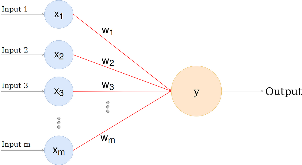
The equation looks like this :

from sklearn.linear_model import Perceptron as skPerceptron
classifier = skPerceptron()
c = classifier.fit(data, labels)

# _new_point = new_point
_new_point = np.random.random(2) 
prediction = c.predict([_new_point])
print(f"point {_new_point} has label: {np.where(prediction==1,'A','B')}")

point [0.4433292  0.40664541] has label: ['A']

plt.scatter(data[:,0],data[:,1],color=color_labels, alpha=0.3)
plt.scatter(_new_point[0],_new_point[1], s=100,c=np.where(prediction==1,color[0],color[1])) # new point
plt.vlines(_new_point[0],_new_point[1]-0.1,_new_point[1]+0.1,'r', alpha=0.5)
plt.hlines(_new_point[1],_new_point[0]-0.1,_new_point[0]+0.1,'r', alpha=0.5)

<matplotlib.collections.LineCollection at 0x7f7d68ee32d0>

class Perceptron(object):
    

    def __init__(self, eta=0.01, n_iter=10):
        self.eta = eta #Learning rate
        self.n_iter = n_iter #number of steps

    def fit(self, X, y):
        """
        Search for optimal weights
        """
        
        # initialize weights to zero? 
        # we could pick random weights, also
        # one more than shape of x features
        
        self.w_ = np.zeros(1 + X.shape[1])
        print(self.w_.shape)
        self.history = []
        self.errors_ = [] 
        
        # loop throught training data
        for i in range(self.n_iter):
            print("Epoch:", i)
            hist = []
            errors = 0 # local error variable (counter, keep track of num err)
        
            for xi, target in zip(X,y):
                # get weight value by applying the learning rate (eta)
                # to the error of our update weight

                # subtract the predicted value from the target (label)
                # only possible diff output are: 0, 2, or -2
                #     zero denotes a correct prediction
                #     2 or -2 denotes an incorrect prediction
                diff = target - self.predict(xi)
                # now, multiply difference error by learning rate
                weight = self.eta * diff
                # set weight vector for each of the feats
                feat_weight = weight * xi
                # increment weights of this particular feature
                self.w_[1:] +=  feat_weight
                # NOTE: first value in weight vector 
                # does not correspond to a particular feature
                # so, update first value with general weight
                self.w_[0] += weight
                # update errors only if difference was mistaken
                if diff != 0:
                    errors += diff
                hist.append(self.w_)
            # append the error counter to errors list
            self.errors_.append(errors)
            self.history.append(hist)
        self.history = np.array(self.history)
        return self

    def sum_input_and_weights(self, X):
        """
        Linear combination of the weights and the feature vector
        """
        summ = np.dot(X, self.w_[1:])
        summ += self.w_[0] # add initial weight

        return summ
    
    def activation(self, x):
        """
        Activation function for positive/negative
        """
        y = np.where(x >= 0.0, 1, -1)

        return y
    
    def predict(self, X):
        
        sum_result = self.sum_input_and_weights(X)
        prediction = self.activation(sum_result)

        return prediction

p = Perceptron(eta=0.01,n_iter=10)

p.fit(data, labels)

(3,)
Epoch: 0
Epoch: 1
Epoch: 2
Epoch: 3
Epoch: 4
Epoch: 5
Epoch: 6
Epoch: 7
Epoch: 8
Epoch: 9

<__main__.Perceptron at 0x7f7d68e9d4d0>

p.predict(np.random.random(2))

array(1)

print(p.errors_)

[0, 0, 0, 0, 0, 0, 0, 0, 0, 0]

p.history.shape
x = np.linspace(0,1,p.n_iter)

_new_point = np.random.random(2) 

prediction = c.predict([_new_point])
custom_prediction = p.predict(_new_point)

print(f"point {_new_point}")
print(f"Sklearn Perceptron: {np.where(prediction==1,'A','B')}")
print(f"Custom Perceptron:  {np.where(custom_prediction==1,'A','B')}")


plt.scatter(data[:,0],data[:,1],color=color_labels, alpha=0.3)

plt.scatter(_new_point[0],_new_point[1], s=100,c=np.where(prediction==1,color[0],color[1])) # new point

plt.vlines(_new_point[0],_new_point[1]-0.1,_new_point[1]+0.1,'r', alpha=0.5)
plt.hlines(_new_point[1],_new_point[0]-0.1,_new_point[0]+0.1,'r', alpha=0.5)

point [0.98957914 0.97579757]
Sklearn Perceptron: ['A']
Custom Perceptron:  A

<matplotlib.collections.LineCollection at 0x7f7d68ee3a50>

plt.scatter(np.random.random(20)*0.1+0.3,np.random.random(20)*0.1+0.3, c=color[0], label='A')
plt.scatter(np.random.random(20)*0.1+0.4,np.random.random(20)*0.1+0.4, c=color[1], label='B')
plt.legend()

<matplotlib.legend.Legend at 0x7f7d68dbc090>

Support Vector Machine (classifier)

The core idea of SVM is to find a maximum marginal line (or hyperplane in multivariate data) that best divides the dataset into classes.

from sklearn import svm
m = svm.SVC(kernel='linear')

m_fitted = m.fit(data, labels)
m_fitted.score(data,labels)

0.96

prediction = m_fitted.predict([new_point])
print(f"point {new_point} has label: {prediction}")

point [0.5, 0.85] has label: [-1]

print(m.classes_) # classes or labels we gave it
print(m.n_support_) # get number of support vectors for each class
print(m.support_) # get indices of support vectors

[-1  1]
[23 23]
[ 4  5  6  8  9 14 15 26 29 30 31 34 35 39 45 49 54 63 66 68 76 93 95  1
 17 23 28 36 37 40 42 43 44 48 51 53 56 58 59 64 79 81 83 85 86 99]

here's a function to plot svc decision function

def plot_svc_decision_function(model, ax=None, plot_support=True):
    """Plot the decision function for a 2D SVC"""
    if ax is None:
        ax = plt.gca()
    xlim = ax.get_xlim()
    ylim = ax.get_ylim()
    
    # create grid to evaluate model
    x = np.linspace(xlim[0], xlim[1], 30)
    y = np.linspace(ylim[0], ylim[1], 30)
    Y, X = np.meshgrid(y, x)
    xy = np.vstack([X.ravel(), Y.ravel()]).T
    P = model.decision_function(xy).reshape(X.shape)
    
    # plot decision boundary and margins
    ax.contour(X, Y, P, colors='k',
               levels=[-1, 0, 1], alpha=0.5,
               linestyles=['--', '-', '--'])
    
    # plot support vectors
    if plot_support:
        ax.scatter(model.support_vectors_[:, 0],
                   model.support_vectors_[:, 1],
                   s=300, linewidth=4, facecolors='grey', alpha=0.2);
    ax.set_xlim(xlim)
    ax.set_ylim(ylim)

#  plot points
plt.scatter(data[:,0],data[:,1],color=color_labels, s=50, alpha=0.8)
#  labelled new point
plt.scatter(new_point[0],new_point[1], color=color[2]) 
#  plot support vectors and decision function
plot_svc_decision_function(m)
# plt.scatter(m.support_vectors_[:,0], m.support_vectors_[:,1], s=300, alpha=0.4, facecolors='grey')

Cross validation

code adapted from: https://colab.research.google.com/github/jakevdp/PythonDataScienceHandbook/blob/master/notebooks/05.07-Support-Vector-Machines.ipynb#scrollTo=JN-t-aHksW1p

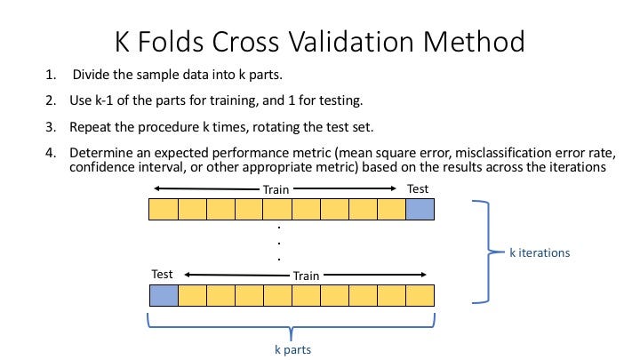
from sklearn.model_selection import train_test_split
 # 70% training and 30% test
print(data.shape, labels.shape)
X_train, X_test, y_train, y_test = train_test_split(data, labels, test_size=0.3,random_state=None)
print("X_train.shape :", X_train.shape )  
print("X_test.shape  :", X_test.shape  )
print("y_train.shape :", y_train.shape )
print("y_test.shape  :", y_test.shape  )
m = svm.SVC()
m_fitted = m.fit(X_train, y_train)
# prediction = m_fitted.predict([new_point])
print("Score:", m.score(X_test,y_test)*100)

(100, 2) (100,)
X_train.shape : (70, 2)
X_test.shape  : (30, 2)
y_train.shape : (70,)
y_test.shape  : (30,)
Score: 93.33333333333333

Finally, we can use a grid search cross-validation to explore combinations of parameters. Here we will adjust C (which controls the margin hardness) and gamma (which controls the size of the radial basis function kernel), and determine the best model:

from sklearn.model_selection import GridSearchCV


param_grid = {'C'    : [1, 5, 10, 50, 55, 25],
              'gamma': [0.0001, 0.0005, 0.001, 0.005, 0.0055, 0.0025]}



grid = GridSearchCV(m, param_grid)

%time grid.fit(X_train, y_train)
print(grid.best_params_)

CPU times: user 228 ms, sys: 0 ns, total: 228 ms
Wall time: 232 ms
{'C': 55, 'gamma': 0.0025}

model = grid.best_estimator_
yfit = model.predict(X_test)

print("Score:", model.score(X_test, y_test)*100)

Score: 96.66666666666667

plt.scatter(X_test[:,0], X_test[:,1], c=np.where(y_test==1,color[0],color[1]))
print(yfit)

[ 1 -1  1 -1 -1 -1  1 -1  1 -1 -1 -1 -1 -1 -1  1  1 -1 -1 -1 -1 -1  1 -1
 -1  1 -1 -1  1  1]

from sklearn.metrics import classification_report
print(classification_report(y_test, yfit,
                            labels=labels, target_names=np.where(y_test==1,'A','B')))

              precision    recall  f1-score   support

           A       0.95      1.00      0.97        19
           B       1.00      0.91      0.95        11
           A       0.95      1.00      0.97        19
           B       1.00      0.91      0.95        11
           B       0.95      1.00      0.97        19
           B       0.95      1.00      0.97        19
           A       0.95      1.00      0.97        19
           B       0.95      1.00      0.97        19
           A       0.95      1.00      0.97        19
           B       0.95      1.00      0.97        19
           B       0.95      1.00      0.97        19
           B       0.95      1.00      0.97        19
           B       1.00      0.91      0.95        11
           B       0.95      1.00      0.97        19
           B       0.95      1.00      0.97        19
           A       0.95      1.00      0.97        19
           A       0.95      1.00      0.97        19
           B       1.00      0.91      0.95        11
           B       0.95      1.00      0.97        19
           B       0.95      1.00      0.97        19
           B       1.00      0.91      0.95        11
           B       1.00      0.91      0.95        11
           A       0.95      1.00      0.97        19
           A       1.00      0.91      0.95        11
           B       0.95      1.00      0.97        19
           A       1.00      0.91      0.95        11
           B       0.95      1.00      0.97        19
           B       0.95      1.00      0.97        19
           A       1.00      0.91      0.95        11
           A       0.95      1.00      0.97        19

    accuracy                           0.97      1564
   macro avg       0.97      0.96      0.97      1564
weighted avg       0.96      0.97      0.97      1564

/usr/local/lib/python3.7/dist-packages/sklearn/metrics/_classification.py:1989: UserWarning: labels size, 100, does not match size of target_names, 30
  .format(len(labels), len(target_names))

from sklearn.metrics import confusion_matrix
import seaborn as sns
mat = confusion_matrix(y_test, yfit)
sns.heatmap(mat.T, square=True, annot=True, cbar=False,
            xticklabels=['A','B'],
            yticklabels=['A','B'])
plt.xlabel('true label')
plt.ylabel('predicted label');

__new_point = np.random.random(2)
_prediction = model.predict([__new_point])
#  plot points
plt.scatter(data[:,0],data[:,1],color=color_labels, s=50)
#  labelled new point
plt.scatter(__new_point[0],__new_point[1], color=np.where(_prediction==1,color[0],color[1])) 
#  plot support vectors and decision function
plot_svc_decision_function(model)
# plt.scatter(m.support_vectors_[:,0], m.support_vectors_[:,1], s=300, alpha=0.4, facecolors='grey')

print(m.support_vectors_ == model.support_vectors_)

False

/usr/local/lib/python3.7/dist-packages/ipykernel_launcher.py:1: DeprecationWarning: elementwise comparison failed; this will raise an error in the future.
  """Entry point for launching an IPython kernel.

Exercise

Prepare data from the the Spotify API (or other sources) so it can be used on a Linear Classifier such as the SVM

# import pandas as pd ?

# load file
# get feature vector (eg, danceability, instrumentality..., etc)
# get labels (eg, artist name,) 
# split data into training, test,